ABaCo tutorial: Inflammatory Bowel Disease case study dataset#
This notebook is a tutorial for implementing ABaCo for data integration of two studies from Inflammatory Bowel Disease (IBD) patients (Crohn’s Disease and Ulcerative Colitis).
Data Description:
The dataset is composed of two different BioProjects which were merged directly before pre-processing: one that studies the dynamics of microbiome functionality in IBD (accession: PRJNA389280) and another that includes multi-omics measurements from IBD patients in a longitudinal study (accession: PRJNA398089).
For consistency, only the genus-level taxa were retained, resulting in a dataset comprising 435 taxonomic groups and 524 samples.
Metadata was retrieved from the Data Repository for Human Gut Microbiota (GMrepo), where the phenotype identifiers were mapped to categorical labeles (i.e. D003425 → Crohn’s Disease, D003093 → Ulcerative Colitis, and D006262 → nonIBD).
Goal:
Using ABaCo the goal is to integrate both datasets without including study-specific technical signals, and only retaining the biological source of variation (IBD vs nonIBD).
Loading the IBD dataset#
abaco provides in dataloader the function DataPreprocess in order to convert plain text file (e.g. csv, tsv, etc.) into pd.DataFrame compatible with ABaCo.
from abaco.dataloader import DataPreprocess, one_hot_encoding

# Load IBD
path_to_data = "data/dataset_ibd.csv"
batch_col = "project ID"
id_col = "run ID"
bio_col = "associated phenotype"

df_ibd = DataPreprocess(
    path_to_data,
    factors=[
        id_col,
        batch_col,
        bio_col
    ]
)
print(df_ibd.info())
<class 'pandas.core.frame.DataFrame'>
RangeIndex: 517 entries, 0 to 516
Columns: 197 entries, run ID to sk__Bacteria;k__;p__Verrucomicrobia;c__Verrucomicrobiae;o__Verrucomicrobiales;f__Akkermansiaceae;g__Akkermansia
dtypes: category(3), float64(193), object(1)
memory usage: 806.2+ KB
None
We can get a summary of the data using with the categorical columns now.
# wrapped summary by project ID
summary_parts = []
for batch in df_ibd[batch_col].cat.categories:
    counts = df_ibd.loc[df_ibd[batch_col] == batch, bio_col].value_counts(dropna=False)
    parts = [f"{ph}: {cnt}" for ph, cnt in counts.items()]
    summary_parts.append(f"{batch_col} - {batch}: " + ", ".join(parts))

print("\n".join(summary_parts))
project ID - PRJNA389280: CD: 175, UC: 97, nonIBD: 69
project ID - PRJNA398089: CD: 85, UC: 46, nonIBD: 45
Using ABaCo#
Training model#
from abaco.ABaCo import metaABaCo
import torch

# defining device
device = torch.device("cuda" if torch.cuda.is_available() else "cpu")

# model definition
model = metaABaCo(
    data=df_ibd,
    n_bios=3,
    bio_label=bio_col,
    n_batches=2,
    batch_label=batch_col,
    n_features=193,
    device=device,
    prior="VMM",
    pdist="ZINB",
    epochs=[4000,1000,2000],
    d_z=32,
)

# fitting model into data
model.fit(
    disc_lr=1e-6,
    adv_lr=1e-6,
    w_bio_penalty=1e-2,
    w_cluster_penalty=1.0,
    phase_1_vae_lr=1e-4,
    phase_2_vae_lr=1e-6,
    phase_3_vae_lr=1e-6,
    w_elbo_kl=1e-3,
    w_elbo_nll=1e-3,
    seed = 42,
    )
Training: VAE for learning meaningful embeddings: 100%|██████████| 4000/4000 [02:02<00:00, 32.71it/s, bio_penalty=0.0009, clustering_loss=0.0005, elbo=0.2231, epoch=3999/4001, vae_loss=0.2244]
Training: Embeddings batch effect correction using adversrial training: 100%|██████████| 1000/1000 [00:34<00:00, 29.37it/s, adv_loss=-0.6930, bio_penalty=0.0009, clustering_loss=0.0000, disc_loss=0.6930, elbo=0.2243, epoch=999/1001, vae_loss=0.2251]
Training: VAE decoder with masked batch labels: 100%|██████████| 2000/2000 [00:35<00:00, 56.62it/s, cycle_loss=0.0000, epoch=2000/2000, vae_loss=0.2355]
Correction with ABaCo trained model#
from abaco.plots import plotPCoA

corrected_dataset = model.correct(seed=42)

plotPCoA(
    data = corrected_dataset,
    sample_label=id_col,
    batch_label=batch_col,
    experiment_label=bio_col,
)
Dealing with outlier runs#
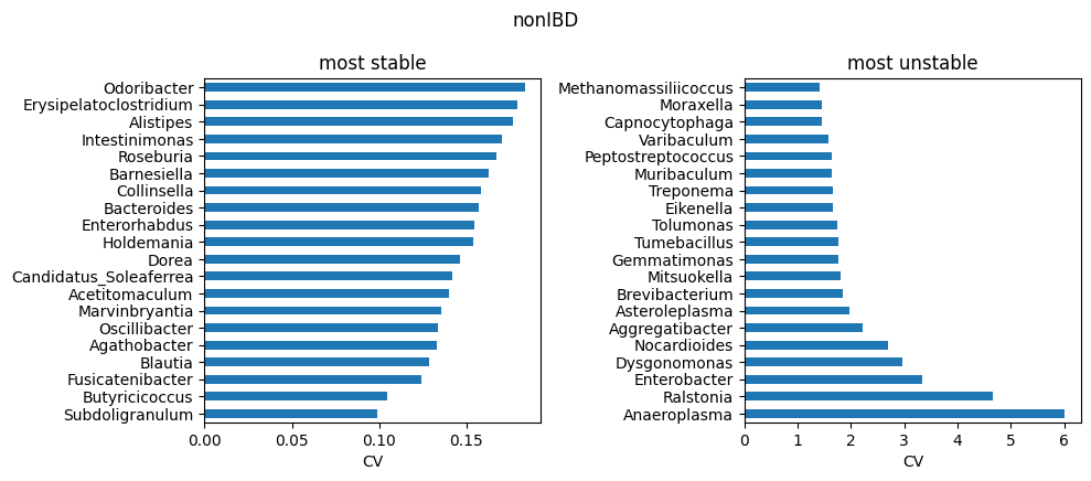
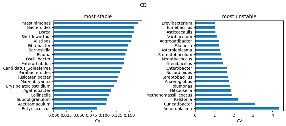
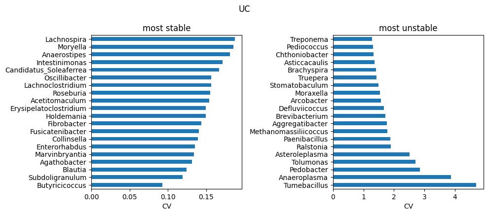
Highly heterogeneous cohorts (e.g. IBD) can produce a small number of extreme outlier runs. In this case, this dataset have been used to train ABaCo 50 different times in order to report robustness. Taxons across runs, specially in samples that are typically more variable across individuals from the same group, are sensible to different initializations or/and hyperparameters. Therefore, analysis of heterogeneous atlases including multiple training replicates can be useful to identify troublesome taxons in the dataset. For each biological group, the run-to-run coefficient of variation for each taxon was computed and saved on data/ibd_taxon_stats/. The most stable and unstable taxons are then reported as follows:
import os, glob
import pandas as pd
import matplotlib.pyplot as plt

def to_genus(t):
    return next((x.replace('g__','') for x in str(t).split(';') if x.startswith('g__')), t)

TOP_K = 20
data_dir = "data/ibd_taxon_stats"

groups = [os.path.basename(p).replace('all_taxa_variability_','').replace('.csv','')
          for p in glob.glob(os.path.join(data_dir, 'all_taxa_variability_*.csv'))]

for g in groups:
    stats = pd.read_csv(os.path.join(data_dir, f'all_taxa_variability_{g}.csv'), index_col=0)
    stable_path   = os.path.join(data_dir, f'stable_taxa_{g}.csv')
    unstable_path = os.path.join(data_dir, f'unstable_taxa_{g}.csv')

    stable   = pd.read_csv(stable_path, index_col=0)   if os.path.exists(stable_path)   else stats.nsmallest(TOP_K, 'cv')
    unstable = pd.read_csv(unstable_path, index_col=0) if os.path.exists(unstable_path) else stats.nlargest(TOP_K, 'cv')

    # to genus
    stats.index    = stats.index.map(to_genus)
    stable.index   = stable.index.map(to_genus)
    unstable.index = unstable.index.map(to_genus)

    # stable vs unstable
    fig, axs = plt.subplots(1, 2, figsize=(10, max(3, 0.22*TOP_K)))
    stable['cv'].head(TOP_K).sort_values().plot.barh(ax=axs[0])
    axs[0].set_title('most stable'); axs[0].set_xlabel('CV')

    unstable['cv'].head(TOP_K).sort_values(ascending=False).plot.barh(ax=axs[1])
    axs[1].set_title('most unstable'); axs[1].set_xlabel('CV')

    plt.suptitle(g)
    plt.tight_layout()
    plt.show()