Report: ABaCo fine-tuning and performance

This notebook has two clear goals:

1. Use a small validation set from the training dataset in order to swiftly optimize the parameters of the model.

2. Report the performance of ABaCo as a function of the number of samples and features of the dataset, in order to estimate the computational cost of running the whole framework.

For these, a simulated dataset with a zero-inflated negative binomial distribution along with both batch and biological effect introduce are used.

---

Data Description:

• The dataset for both analyses are generated using the zinb_simulated() function, which works in the same way as described in the ABaCo paper.

• Two biological groups and two batches are used on these, with a proportion of 50/50 on the biology distribution and 60/40 on the batches to simulate a small unbalance.

---

Zero-inflated Negative Binomial Simulated data

To get the ZINB-like simulated data we define the zinb_simulated() function:

import numpy as np
import pandas as pd
from scipy.stats import nbinom


def zinb_simulated(
    n_samples=200,
    n_features=1000,
    p_diff=0.5,
    b_diff=0.1,
    sims=1,
    bio_prop=[0.5, 0.5],
    batch_prop=[0.6, 0.4],
    seed=42,
):

    # ── 0. Reproducibility & basic parameters ─────────────────────────────────────
    np.random.seed(seed)

    n_diff = int(n_features * p_diff)
    n_bdiff = int(n_features * b_diff)

    bios = ["A", "B"]
    batches = ["Batch 1", "Batch 2"]

    sim_data_bt = []
    sim_data_gt = []


    # ── Global feature‐level params ────────────────────────────────────────────────
    r = np.random.uniform(1, 3, size=n_features)
    baseline_log = np.random.normal(2, 1, size=n_features)

    # zero-inflation
    high_zero_prop = int(
        n_features * 0.7
    )  # 70% of features being sparse with over-inflation of zeroes
    low_zero_prop = n_features - high_zero_prop

    high_zero = np.random.uniform(0.8, 0.9, high_zero_prop)
    low_zero = np.random.uniform(0.1, 0.8, low_zero_prop)

    z_target = np.concatenate([high_zero, low_zero])

    mu0 = np.exp(baseline_log)
    p_nb_zero = (r / (r + mu0)) ** r
    p_zero = np.clip((z_target - p_nb_zero) / (1 - p_nb_zero), 0, 1)

    # biological effects
    effect_sizes = np.zeros(n_features)
    idx_diff = np.random.choice(n_features, n_diff, replace=False)
    effect_sizes[idx_diff] = np.random.normal(2, 2, size=n_diff)
    effect_mult = 1 + 0.5 * (effect_sizes / effect_sizes.max())

    # batch effects
    batch_shift = np.zeros(n_features)
    idx_bdiff = np.random.choice(n_features, n_bdiff, replace=False)
    batch_shift[idx_bdiff] = np.random.normal(1, 2, size=n_bdiff)

    # heteroskedastic dispersion & zero‐inflation shifts by batch
    delta_disp = np.random.normal(0, 0.2, size=n_features)
    delta_zero = np.random.normal(0, 0.2, size=n_features)

    # bio×batch interaction
    idx_inter = np.random.choice(n_features, int(0.2 * n_features), replace=False)
    effect_int = np.zeros(n_features)
    effect_int[idx_inter] = np.random.normal(3, 1, size=idx_inter.size)

    # ── Simulation loop ────────────────────────────────────────────────────────────
    for sim in range(sims):
        # 1. Build metadata (no Plate or Age anymore)
        meta = pd.DataFrame(
            {
                "SampleID": [f"S{sim:02d}_{i+1}" for i in range(n_samples)],
                "Condition": np.random.choice(bios, size=n_samples, p=bio_prop),
                "Batch": np.random.choice(batches, size=n_samples, p=batch_prop),
            }
        )

        # placeholders for each scenario
        cnt_bt = np.zeros((n_samples, n_features), dtype=int)
        cnt_gt = np.zeros((n_samples, n_features), dtype=int)

        for i, row in meta.iterrows():
            cond = 1 if row.Condition == "B" else 0
            bat = 1 if row.Batch == "Batch 2" else 0

            # baseline log‐scale
            mu_log_base = baseline_log.copy()

            # --- Scenario 1: ground truth (no batch effect) ---
            mu_log3 = mu_log_base + cond * effect_sizes
            mu3 = np.exp(mu_log3)
            use_m = np.random.rand(n_features) < 0.3
            mu3[use_m] *= 1 + cond * effect_mult[use_m]
            p3 = r / (r + mu3)
            z3 = np.random.binomial(1, p_zero)
            samp3 = nbinom(r, p3).rvs(size=n_features)
            cnt_gt[i] = np.where(z3, 0, samp3)

            # --- Scenario 2: batch + bio + interaction ---
            mu_log4 = (
                mu_log_base
                + cond * effect_sizes
                + bat * batch_shift
                + cond * bat * effect_int
            )
            mu4 = np.exp(mu_log4)
            mu4[use_m] *= 1 + cond * effect_mult[use_m]
            r4 = r * (1 + bat * delta_disp)
            p04 = np.clip(p_zero * (1 + bat * delta_zero), 0, 1)
            p4 = r4 / (r4 + mu4)
            z4 = np.random.binomial(1, p04)
            samp4 = nbinom(r4, p4).rvs(size=n_features)

            cnt_bt[i] = np.where(z4, 0, samp4)

        cols = [f"OTU{j+1}" for j in range(n_features)]

        sim_data_bt.append(
            pd.concat([meta, pd.DataFrame(cnt_bt, columns=cols)], axis=1)
        )

        sim_data_gt.append(
            pd.concat([meta, pd.DataFrame(cnt_gt, columns=cols)], axis=1)
        )
    
    return sim_data_bt, sim_data_gt

Principal Coordinate Analysis Plot

We are going to use a custom PCoA plot function in order to visualize the data better:

from scipy.spatial.distance import pdist, squareform
from skbio.stats.distance import DistanceMatrix, permanova
from skbio.stats.ordination import pcoa
import matplotlib.pyplot as plt
from matplotlib.patches import Ellipse
from matplotlib.gridspec import GridSpec
from mpl_toolkits.axes_grid1 import make_axes_locatable
import seaborn as sns
import pandas as pd
import numpy as np

# Auxiliary
def permanova_ait(df, sample_label, group_label):
    samples = df[sample_label].values
    groups = df[group_label].values
    clr_data = df.select_dtypes(include = "number").values

    aitch = pdist(clr_data, metric = "euclidean")
    dist_mat = squareform(aitch)
    dm = DistanceMatrix(dist_mat, ids=samples)

    res_ait = permanova(distance_matrix=dm, grouping=groups)

    res_ait["R2"] = (
        res_ait["test statistic"]
        * (len(np.unique(groups)) - 1)
        / (
            res_ait["test statistic"] * (len(np.unique(groups)) - 1)
            + (len(samples) - len(np.unique(groups)))
        )
    )
    return res_ait

def pcoa_aitchison(df, sample_label, batch_label, bio_label):
    df_otu = df.select_dtypes(include="number")
    dist = pdist(df_otu, "euclidean")
    dist = squareform(dist)

    pcoa_res = pcoa(dist)
    explained = (pcoa_res.proportion_explained * 100).round(1)
    explained_dict = {"PC1": explained[0], "PC2": explained[1]}
    df_pcoa = pd.DataFrame(pcoa_res.samples[["PC1","PC2"]], columns=["PC1","PC2"])
    df_pcoa.index = (
        df.index
    )
    df_pcoa[[sample_label, batch_label, bio_label]] = df[[sample_label, batch_label, bio_label]]
    return df_pcoa, explained_dict

def plot_pcoa_2(
    df_pcoa,
    group_col,
    df,
    sample_label,
    ax,
    explained,
    palette=None,
    xlim=None,
    ylim=None,
    marginal_size="20%",     # size of marginals relative to main
    marginal_pad=0.1,         # padding between main and marginals
    kde_bw_adjust=1.0,        # bandwidth scaling for KDE
    alpha_kde=0.5,            # fill transparency for KDE areas
    title=None,               # optional title above the top density plot
    show_legend=True          # whether to draw the legend
):
    # compute PERMANOVA R2
    perma_r2 = permanova_ait(df, sample_label, group_col)["R2"]

    # set up axes divider for marginals
    divider = make_axes_locatable(ax)
    ax_top   = divider.append_axes("top",    size=marginal_size, pad=marginal_pad, sharex=ax)
    ax_right = divider.append_axes("right",  size=marginal_size, pad=marginal_pad, sharey=ax)

    # hide the marginal axes completely (no ticks, no spines)
    ax_top.axis('off')
    ax_right.axis('off')

    groups = df_pcoa[group_col].unique()
    colors = palette or plt.cm.tab10.colors

    handles = []
    labels  = []

    for i, grp in enumerate(groups):
        sub = df_pcoa[df_pcoa[group_col] == grp]
        x = sub['PC1'].values
        y = sub['PC2'].values
        c = colors[i % len(colors)]

        # main scatter
        pts = ax.scatter(x, y, label=str(grp), alpha=0.7, color=c)
        handles.append(pts)
        labels.append(str(grp))

        # marginal KDEs (axes are off so only the filled area shows)
        sns.kdeplot(
            x=x, ax=ax_top, bw_adjust=kde_bw_adjust,
            fill=True, alpha=alpha_kde, color=c, linewidth=1.5
        )
        sns.kdeplot(
            y=y, ax=ax_right, bw_adjust=kde_bw_adjust,
            fill=True, alpha=alpha_kde, color=c, linewidth=1.5
        )

        # 95% confidence ellipse
        cov = np.cov(x, y)
        vals, vecs = np.linalg.eigh(cov)
        width, height = 2 * np.sqrt(vals * 5.991)
        angle = np.degrees(np.arctan2(*vecs[:,0][::-1]))
        ell = Ellipse(
            xy=(x.mean(), y.mean()),
            width=width, height=height,
            angle=angle, edgecolor=c, facecolor='none', lw=2
        )
        ax.add_patch(ell)

    # add title above the top density plot
    if title:
        ax_top.set_title(title, pad=10, fontsize=16)

    # optionally draw legend on top density axis
    if show_legend:
        ax_top.legend(
            handles, labels,
            title=group_col,
            bbox_to_anchor=(1.02, 1), loc='upper left',
            frameon=False,
            fontsize=14,
            title_fontsize=16,
        )

    # main axis formatting
    ax.set_xlabel(f"PC1 ({explained['PC1']:.1f}%)", fontsize=12)
    ax.set_ylabel(f"PC2 ({explained['PC2']:.1f}%)", fontsize=12)
    ax.text(
        0.99, 0.99,
        f"PERMANOVA R² ({group_col}): {perma_r2:.3f}",
        transform=ax.transAxes, ha="right", va="top", fontsize="small"
    )
    ax.set_aspect('equal')

    if xlim is not None:
        ax.set_xlim(xlim)
    if ylim is not None:
        ax.set_ylim(ylim)

Validation set for weights fine-tuning

To get started with ABaCo, selecting the correct weights to train the model is fundamental for having a good balance between batch correction and biological conservation. However, finding the correct set of weights on the whole dataset can result in a slow process due to training time. Therefore, we can select a small subset of around 10-20% of the whole training set to find the correct weights for the model.

First, we create the simulated ZINB-like data with zinb_simulated():

bt, gt = zinb_simulated()

bt is the simulated data with the batch effect, while gt in this case is the ground-truth without any batch effect. We can visualize this with pcoa_aitchison and plot_pcoa_2():

# Define figure
from abaco.dataloader import DataTransform

sns.set_style("whitegrid")
fig = plt.figure(figsize=(24, 20))
fig.suptitle("", fontsize=16, y=0.97)

gs = GridSpec(2, 2, figure=fig, wspace=0.4, hspace=0.2)

top_palette = sns.color_palette("tab10", n_colors=9)
bottom_palette = sns.color_palette("tab10", n_colors=10)[::-1][:9]

ax1 = fig.add_subplot(gs[0,0])
ax2 = fig.add_subplot(gs[0,1])
ax3 = fig.add_subplot(gs[1,0])
ax4 = fig.add_subplot(gs[1,1])

id_col = "SampleID"
batch_col = "Batch"
bio_col = "Condition"
data_gt_clr = DataTransform(gt[0], factors=[id_col, batch_col, bio_col], count=True)
data_bt_clr = DataTransform(bt[0], factors=[id_col, batch_col, bio_col], count=True)
data_clr = [data_gt_clr, data_bt_clr]
axes=[[ax1, ax2], [ax3, ax4]]

for i, data in enumerate(data_clr):

    data_pcoa, data_exp = pcoa_aitchison(
        data,
        sample_label=id_col,
        batch_label=batch_col,
        bio_label=bio_col
    )

    plot_pcoa_2(
        data_pcoa,
        group_col=batch_col,
        df=data,
        sample_label=id_col,
        ax=axes[i][0],
        explained=data_exp,
        palette=top_palette,
        title="Aitchison PCoA - Colored by Study",
        show_legend=False,
        xlim=[-45,50],
        ylim=[-45,45]
    )

    handles, labels = axes[i][0].get_legend_handles_labels()

    fig.legend(
        handles, labels,
        title="Batch",
        loc = "upper right",
        frameon = False,
        bbox_to_anchor = (0.46, 0.55),
        fontsize=14,
        title_fontsize=14
    )

    plot_pcoa_2(
        data_pcoa,
        group_col=bio_col,
        df=data,
        sample_label=id_col,
        ax=axes[i][1],
        explained=data_exp,
        palette=bottom_palette,
        title="Aitchison PCoA - Colored by Phenotype",
        show_legend=False,
        xlim=[-45,50],
        ylim=[-45,45]
    )

    handles, labels = axes[i][1].get_legend_handles_labels()

    fig.legend(
        handles, labels,
        title="Phenotype",
        loc = "upper right",
        frameon = False,
        bbox_to_anchor = (0.87, 0.55),
        fontsize=14,
        title_fontsize=14
    )

    # Add row title on the left
    row_title = "Ground Truth Dataset" if i == 0 else "Dataset with Batch Effect"
    fig.text(0.07, 0.67 - i*0.42, row_title, va='center', fontsize=18, rotation=90)

fig.subplots_adjust(right=0.85)

plt.show()

/tmp/ipykernel_3996212/2689478418.py:41: FutureWarning: Series.__getitem__ treating keys as positions is deprecated. In a future version, integer keys will always be treated as labels (consistent with DataFrame behavior). To access a value by position, use `ser.iloc[pos]`
  explained_dict = {"PC1": explained[0], "PC2": explained[1]}
/tmp/ipykernel_3996212/2689478418.py:41: FutureWarning: Series.__getitem__ treating keys as positions is deprecated. In a future version, integer keys will always be treated as labels (consistent with DataFrame behavior). To access a value by position, use `ser.iloc[pos]`
  explained_dict = {"PC1": explained[0], "PC2": explained[1]}

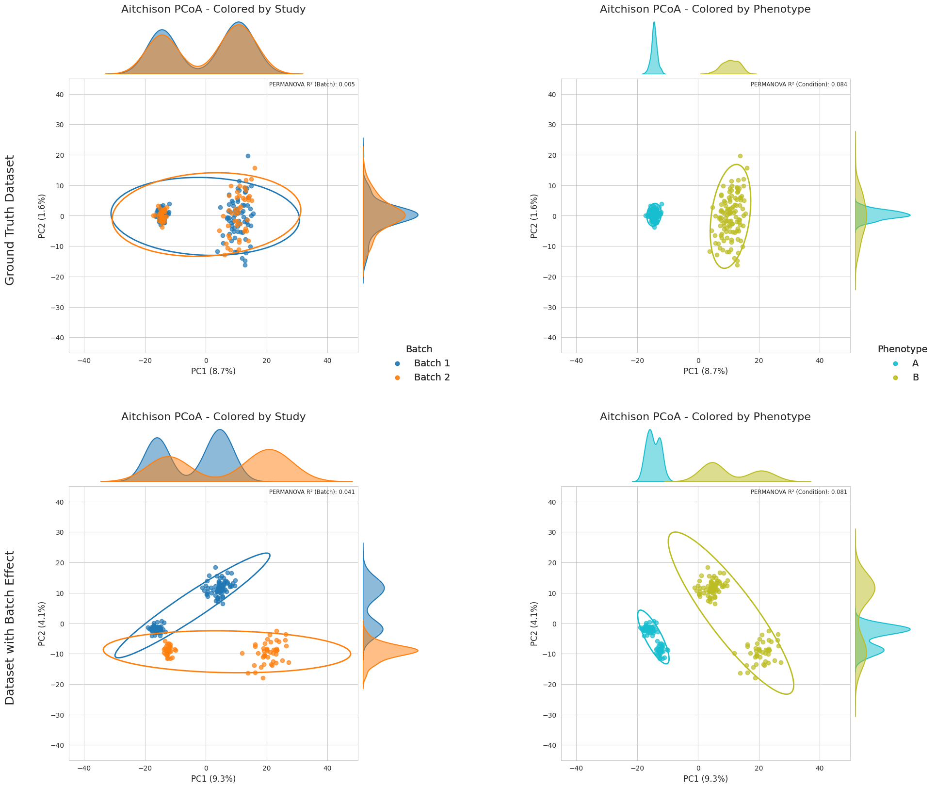
There’s clearly a batch effect in this simulated dataset which, compared to the ground-truth, adds a lot of bias into the data. For fine-tuning the weights and testing different configurations in a fast way, we are going to sample 20% of the data:

import numpy as np

val_prop = 0.2 # 20% validation
dataset = bt[0]
val_set = dataset.groupby(['Condition', 'Batch'], group_keys=False).apply(
    lambda g: g.sample(n=max(1, int(np.ceil(len(g) * val_prop))), random_state=42)
).reset_index(drop=True)

/tmp/ipykernel_3996212/4041600969.py:5: FutureWarning: DataFrameGroupBy.apply operated on the grouping columns. This behavior is deprecated, and in a future version of pandas the grouping columns will be excluded from the operation. Either pass `include_groups=False` to exclude the groupings or explicitly select the grouping columns after groupby to silence this warning.
  val_set = dataset.groupby(['Condition', 'Batch'], group_keys=False).apply(

Now we are going to use the metaABaCo() from abaco.ABaCo to define the model and start training it with the fit() method:

from abaco.ABaCo import metaABaCo
import torch

batch_col = "Batch"
bio_col = "Condition"
id_col = "SampleID"

device = torch.device("cuda" if torch.cuda.is_available() else "cpu")

# Create ABaCo model
abaco_model = metaABaCo(
    data = val_set,
    n_bios = 2,
    bio_label = bio_col,
    n_batches=2,
    batch_label=batch_col,
    n_features=val_set.select_dtypes(include="number").shape[1],
    prior="VMM",
    device=device,
    epochs=[5000, 2000, 1000]
)

abaco_model.fit(seed=42,
                w_cluster_penalty=10.0,
                w_bio_penalty=10.0,
                w_elbo_kl=10.0,
                phase_1_vae_lr=2e-4,
                phase_2_vae_lr=1e-6,
                phase_3_vae_lr=1e-6,
                disc_lr=1e-7,
                adv_lr=1e-7)

Training: VAE for learning meaningful embeddings: 100%|██████████| 5000/5000 [02:15<00:00, 36.96it/s, bio_penalty=0.0001, clustering_loss=0.0005, elbo=4596.2451, epoch=4999/5001, vae_loss=4596.2456]    
Training: Embeddings batch effect correction using adversrial training: 100%|██████████| 2000/2000 [00:46<00:00, 43.46it/s, adv_loss=-0.6888, bio_penalty=0.0000, clustering_loss=0.0000, disc_loss=0.6888, elbo=1483.1102, epoch=1999/2001, vae_loss=1483.1102]
Training: VAE decoder with masked batch labels: 100%|██████████| 1000/1000 [00:08<00:00, 112.43it/s, cycle_loss=0.0000, epoch=1000/1000, vae_loss=1426.0414]

And to check if the current weights are suitable for our dataset, we can have a fast check of the reconstructed data using the PCoA plot:

# Define figure
val_corrected = abaco_model.correct(seed=42)

sns.set_style("whitegrid")
fig = plt.figure(figsize=(24, 20))
fig.suptitle("", fontsize=16, y=0.97)

gs = GridSpec(2, 2, figure=fig, wspace=0.4, hspace=0.2)

top_palette = sns.color_palette("tab10", n_colors=9)
bottom_palette = sns.color_palette("tab10", n_colors=10)[::-1][:9]

ax1 = fig.add_subplot(gs[0,0])
ax2 = fig.add_subplot(gs[0,1])
ax3 = fig.add_subplot(gs[1,0])
ax4 = fig.add_subplot(gs[1,1])

id_col = "SampleID"
batch_col = "Batch"
bio_col = "Condition"
data_gt_clr = DataTransform(gt[0], factors=[id_col, batch_col, bio_col], count=True)
val_corrected_clr = DataTransform(val_corrected, factors=[id_col, batch_col, bio_col], count=True)
data_clr = [data_gt_clr, val_corrected_clr]
axes=[[ax1, ax2], [ax3, ax4]]

for i, data in enumerate(data_clr):

    data_pcoa, data_exp = pcoa_aitchison(
        data,
        sample_label=id_col,
        batch_label=batch_col,
        bio_label=bio_col
    )

    plot_pcoa_2(
        data_pcoa,
        group_col=batch_col,
        df=data,
        sample_label=id_col,
        ax=axes[i][0],
        explained=data_exp,
        palette=top_palette,
        title="Aitchison PCoA - Colored by Study",
        show_legend=False,
        xlim=[-45,50],
        ylim=[-45,45]
    )

    handles, labels = axes[i][0].get_legend_handles_labels()

    fig.legend(
        handles, labels,
        title="Batch",
        loc = "upper right",
        frameon = False,
        bbox_to_anchor = (0.46, 0.55),
        fontsize=14,
        title_fontsize=14
    )

    plot_pcoa_2(
        data_pcoa,
        group_col=bio_col,
        df=data,
        sample_label=id_col,
        ax=axes[i][1],
        explained=data_exp,
        palette=bottom_palette,
        title="Aitchison PCoA - Colored by Phenotype",
        show_legend=False,
        xlim=[-45,50],
        ylim=[-45,45]
    )

    handles, labels = axes[i][1].get_legend_handles_labels()

    fig.legend(
        handles, labels,
        title="Phenotype",
        loc = "upper right",
        frameon = False,
        bbox_to_anchor = (0.87, 0.55),
        fontsize=14,
        title_fontsize=14
    )

    # Add row title on the left
    row_title = "Ground Truth Dataset" if i == 0 else "ABaCo Corrected Validation Dataset"
    fig.text(0.07, 0.67 - i*0.42, row_title, va='center', fontsize=18, rotation=90)

fig.subplots_adjust(right=0.85)

plt.show()

/tmp/ipykernel_3996212/2689478418.py:41: FutureWarning: Series.__getitem__ treating keys as positions is deprecated. In a future version, integer keys will always be treated as labels (consistent with DataFrame behavior). To access a value by position, use `ser.iloc[pos]`
  explained_dict = {"PC1": explained[0], "PC2": explained[1]}
/tmp/ipykernel_3996212/2689478418.py:41: FutureWarning: Series.__getitem__ treating keys as positions is deprecated. In a future version, integer keys will always be treated as labels (consistent with DataFrame behavior). To access a value by position, use `ser.iloc[pos]`
  explained_dict = {"PC1": explained[0], "PC2": explained[1]}

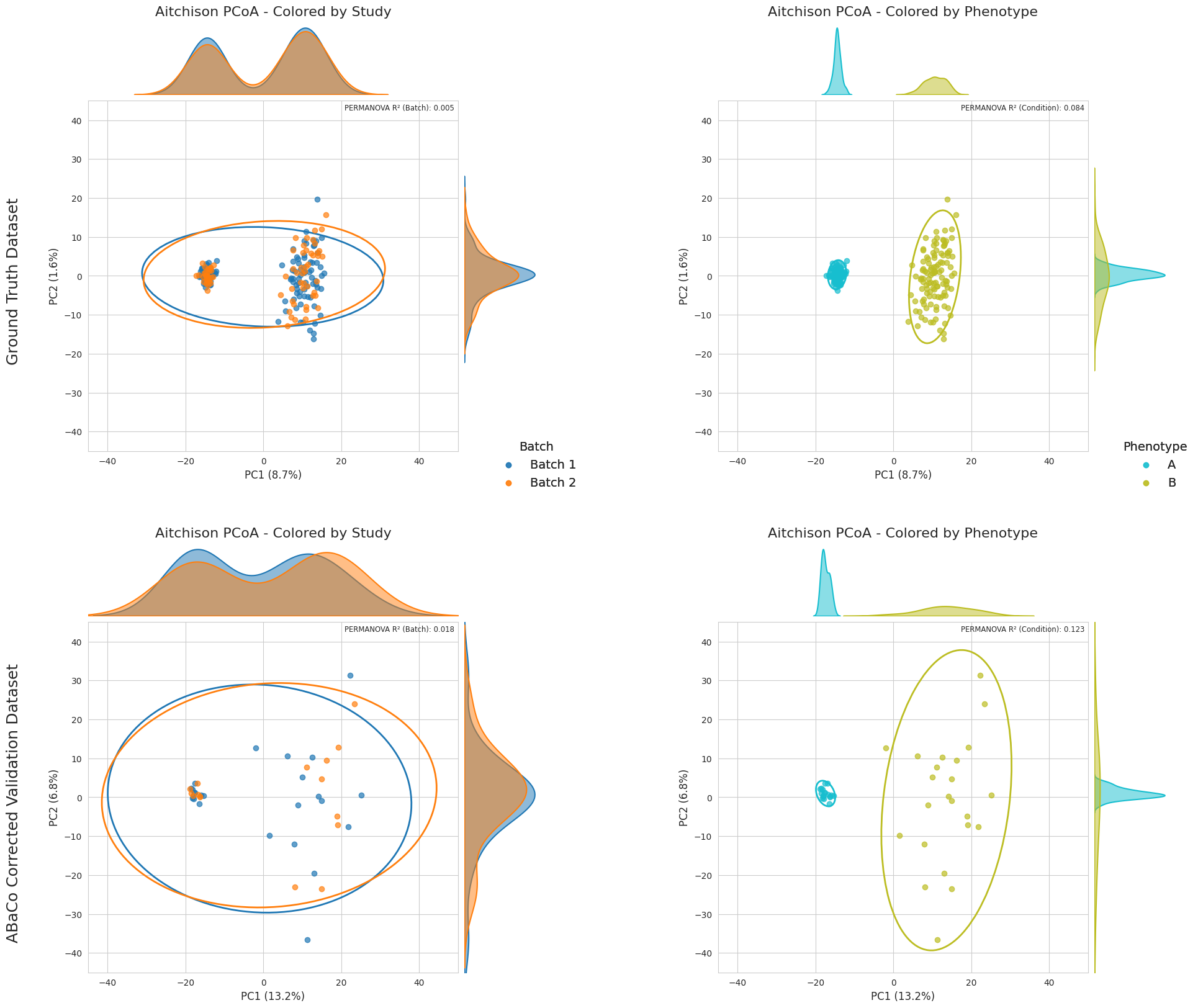
In this case we can see that the corrected model for the validation set presents a considerable higher variance in PC2, but the biological groups separation is preserved and the batch correction successfully done. We are now going to test if these weights are suitable when training with the whole dataset:

from abaco.ABaCo import metaABaCo
import torch

batch_col = "Batch"
bio_col = "Condition"
id_col = "SampleID"

device = torch.device("cuda" if torch.cuda.is_available() else "cpu")

# Create ABaCo model
abaco_model = metaABaCo(
    data = bt[0],
    n_bios = 2,
    bio_label = bio_col,
    n_batches=2,
    batch_label=batch_col,
    n_features=bt[0].select_dtypes(include="number").shape[1],
    prior="VMM",
    device=device,
    epochs=[5000, 2000, 1000]
)

abaco_model.fit(seed=42,
                w_cluster_penalty=10.0,
                w_bio_penalty=10.0,
                w_elbo_kl=10.0,
                phase_1_vae_lr=2e-4,
                phase_2_vae_lr=1e-6,
                phase_3_vae_lr=1e-6,
                disc_lr=1e-7,
                adv_lr=1e-7)

Training: VAE for learning meaningful embeddings: 100%|██████████| 5000/5000 [01:41<00:00, 49.45it/s, bio_penalty=1.1947, clustering_loss=0.0035, elbo=1668.4307, epoch=4999/5001, vae_loss=1669.6288]     
Training: Embeddings batch effect correction using adversrial training: 100%|██████████| 2000/2000 [00:44<00:00, 44.89it/s, adv_loss=-0.7125, bio_penalty=1.1878, clustering_loss=0.0000, disc_loss=0.7125, elbo=1665.6492, epoch=1999/2001, vae_loss=1666.8370]
Training: VAE decoder with masked batch labels: 100%|██████████| 1000/1000 [00:11<00:00, 87.83it/s, cycle_loss=0.0000, epoch=1000/1000, vae_loss=1719.7050]

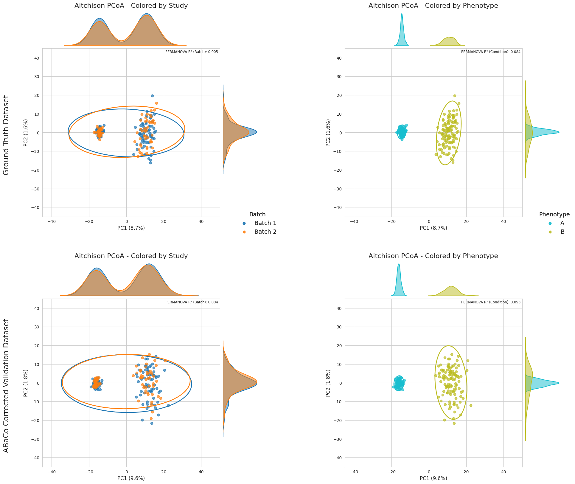
Now we verify the results by doing a final PCoA plot compared to the ground-truth:

# Define figure
all_corrected = abaco_model.correct(seed=42)

sns.set_style("whitegrid")
fig = plt.figure(figsize=(24, 20))
fig.suptitle("", fontsize=16, y=0.97)

gs = GridSpec(2, 2, figure=fig, wspace=0.4, hspace=0.2)

top_palette = sns.color_palette("tab10", n_colors=9)
bottom_palette = sns.color_palette("tab10", n_colors=10)[::-1][:9]

ax1 = fig.add_subplot(gs[0,0])
ax2 = fig.add_subplot(gs[0,1])
ax3 = fig.add_subplot(gs[1,0])
ax4 = fig.add_subplot(gs[1,1])

id_col = "SampleID"
batch_col = "Batch"
bio_col = "Condition"
data_gt_clr = DataTransform(gt[0], factors=[id_col, batch_col, bio_col], count=True)
all_corrected_clr = DataTransform(all_corrected, factors=[id_col, batch_col, bio_col], count=True)
data_clr = [data_gt_clr, all_corrected_clr]
axes=[[ax1, ax2], [ax3, ax4]]

for i, data in enumerate(data_clr):

    data_pcoa, data_exp = pcoa_aitchison(
        data,
        sample_label=id_col,
        batch_label=batch_col,
        bio_label=bio_col
    )

    plot_pcoa_2(
        data_pcoa,
        group_col=batch_col,
        df=data,
        sample_label=id_col,
        ax=axes[i][0],
        explained=data_exp,
        palette=top_palette,
        title="Aitchison PCoA - Colored by Study",
        show_legend=False,
        xlim=[-45,50],
        ylim=[-45,45]
    )

    handles, labels = axes[i][0].get_legend_handles_labels()

    fig.legend(
        handles, labels,
        title="Batch",
        loc = "upper right",
        frameon = False,
        bbox_to_anchor = (0.46, 0.55),
        fontsize=14,
        title_fontsize=14
    )

    plot_pcoa_2(
        data_pcoa,
        group_col=bio_col,
        df=data,
        sample_label=id_col,
        ax=axes[i][1],
        explained=data_exp,
        palette=bottom_palette,
        title="Aitchison PCoA - Colored by Phenotype",
        show_legend=False,
        xlim=[-45,50],
        ylim=[-45,45]
    )

    handles, labels = axes[i][1].get_legend_handles_labels()

    fig.legend(
        handles, labels,
        title="Phenotype",
        loc = "upper right",
        frameon = False,
        bbox_to_anchor = (0.87, 0.55),
        fontsize=14,
        title_fontsize=14
    )

    # Add row title on the left
    row_title = "Ground Truth Dataset" if i == 0 else "ABaCo Corrected Validation Dataset"
    fig.text(0.07, 0.67 - i*0.42, row_title, va='center', fontsize=18, rotation=90)

fig.subplots_adjust(right=0.85)

plt.show()

/tmp/ipykernel_3996212/2689478418.py:41: FutureWarning: Series.__getitem__ treating keys as positions is deprecated. In a future version, integer keys will always be treated as labels (consistent with DataFrame behavior). To access a value by position, use `ser.iloc[pos]`
  explained_dict = {"PC1": explained[0], "PC2": explained[1]}
/tmp/ipykernel_3996212/2689478418.py:41: FutureWarning: Series.__getitem__ treating keys as positions is deprecated. In a future version, integer keys will always be treated as labels (consistent with DataFrame behavior). To access a value by position, use `ser.iloc[pos]`
  explained_dict = {"PC1": explained[0], "PC2": explained[1]}

ABaCo Computational Requirements estimation

In this section, we provide a benchmark analysis of ABaCo’s computational performance. While adversarial generative models can be computationally demanding, it is essential to assess the feasibility of the method for typical research environments. We report the training runtime and peak GPU memory usage across varying dataset sizes and dimensions.

We evaluated the model’s scalability by performing a grid search over dataset dimensions. Let \(N\) denote the number of samples and \(P\) the number of features. We varied \(N \in \{50, \dots, 1000\}\) and \(P \in \{50, \dots, 1000\}\). For each combination of \((N, P)\), we performed 5 independent training runs to capture variability in initialization and during training. All experiments were conducted on a a dual-socket Intel Xeon Gold 6226R server running in x86_64 mode with VT-x virtualization enabled (see ABaCo’s paper, Section 4.5 for more details).

import numpy as np
import pandas as pd
import matplotlib.pyplot as plt
import seaborn as sns

# choose metric
metric = 'wall_s'

# load data
path = "data/abaco_performance_interpolation_iter.csv"
df = pd.read_csv(path)

sns.set_style("whitegrid")
sns.set_context("paper", font_scale=1.4)

# Subplot
fig, axes = plt.subplots(1, 2, figsize=(16, 6))

# --- Plot 1: Runtime Analysis ---
sns.lineplot(
    data=df, 
    x="n_samples", 
    y="wall_s", 
    hue="n_features", 
    palette="viridis",      
    marker="o",             
    ax=axes[0]
)

axes[0].set_title("Computational Time Scalability")
axes[0].set_xlabel("Number of Samples")
axes[0].set_ylabel("Wall Time (seconds)")
axes[0].legend(title="Number of Features")

# --- Plot 2: Memory Usage Analysis ---
sns.lineplot(
    data=df, 
    x="n_samples", 
    y="peak_gpu_gib", 
    hue="n_features", 
    palette="viridis",        
    marker="s",             
    ax=axes[1]
)

axes[1].set_title("GPU Memory Requirements")
axes[1].set_xlabel("Number of Samples")
axes[1].set_ylabel("Peak GPU Memory (GiB)")
axes[1].legend(title="Number of Features")

# Adjust layout and save
plt.tight_layout()
plt.show()

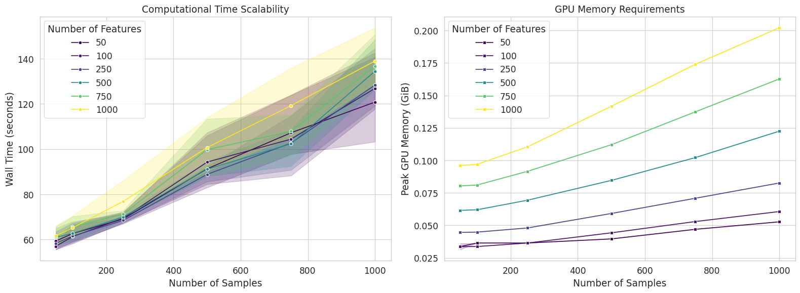
The figure above represents the computational resources assessment of ABaCo:

• Left: Wall-clock training time (seconds) versus number of samples, stratified by number of features (colors). Solid lines represent the mean over 5 independent runs, while shaded regions denote the 95% confidence interval, illustrating training stability.

• Right: Peak GPU memory usage (GiB) versus number of samples. The model exhibits a highly efficient memory footprint, peaking at approximately \(0.20\) GiB for the largest dataset tested (\(N=1000, P=1000\)).

Runtime Scalability:

The wall-clock time required for model training is primarily driven by the number of samples (\(N\)), with the number of features (\(P\)) having a comparatively minor impact on runtime. As shown in Figure \ref{fig:abaco_performance} (left panel), the trajectories for varying feature dimensions (\(P \in [50, 1000]\)) overlap significantly, indicating that the computational cost of the encoder and discriminator networks is dominated by batch processing rather than the input layer width. Overall, the training time \(T(N)\) scales linearly with sample size:

\[\begin{equation*} T(N) \propto \mathcal{O}(N) \end{equation*}\]

For the largest configuration tested (\(N=1000, P=1000\)), the mean training time was approximately \(140\) seconds (\(\approx 2.3\) minutes). Across runs we can see variability in the training time, which is expected given the stochastic nature of adversarial optimization. Despite this, the computational cost remains predictable and linear, ensuring feasibility for larger datasets.

Memory Requirements:

We monitored the peak GPU memory (VRAM) usage during the training phase. The memory footprint of ABaCo is notably low. For the maximum complexity tested (\(N=1000, P=1000\)), the peak VRAM usage was approximately 0.2 GiB. This low memory requirement (\(< 1\) GiB) confirms that ABaCo does not require high-performance enterprise GPUs (e.g., A100) and is fully compatible with standard consumer-grade hardware. The linear scaling of memory usage suggests that the model can process significantly larger batches (e.g., \(N \gg 1000\)) on typical GPUs with 8-12 GiB of VRAM without encountering memory exhaustion.